---- DATABASE ERROR ----

Digging Deep: Parametric Objects

by Mike Kost

Introduction

Povray parametric objects provide a powerful way to create unusual surfaces. Unfortunately, there's very little information out on the Internet describing parametric objects. Hopefully this Digging Deep article will provide a springboard to help people get started using parametric objects in Povray 3.6.

Quick Reading

Here's some reading material on topics that this article will cover

Before Getting Into It

This tutorial will not cover isosurface topics like gradients and bounding boxes. If you're unfamiliar with isosurfaces, try these websites for more information:

Parametric Object Basics

Parametric objects require a bit of brain bending. With parametric objects, two variables are created, u and v, that can be swept from any range. From u and v, we calculate the x, y, and z coordinates represented by every possible u and v value. This defines the surface of the object.

Ummm... Huh?

Lets consider the situation where we say that u is the x coordinate and v is the z coordinate. The y coordinate will be calculated as sin(5*u) and we want a surface that goes from <-1,0,-1> to <1,0,1>. Here's what the Povray code and result would look like:

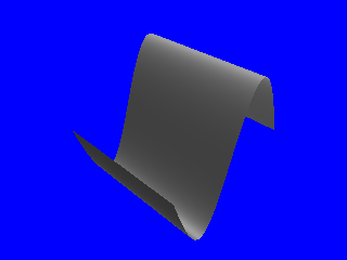
#declare Fx = function { u };
#declare Fy = function { sin(pi*u) };
#declare Fz = function { v };

#declare maxG = 2;

#declare startU = -1;
#declare startV = -1;
#declare endU = 1;
#declare endV = 1;

parametric {
    function { Fx(u,v,0) },
    function { Fy(u,v,0) },
    function { Fz(u,v,0 },
    <startU, startV>, <endU, endV>
    contained_by { box {<-1,-1,-1>,<1,1,1>} }
    max_gradient maxG
    pigment { rgb 0.9 }
    finish { phong 0.5 phong_size 10 }
}

Full source
Example 1 Rendering
The parametric object, in essence, renders the object by sweeping x from -1 to 1, z from -1 to 1, and calculating y = sin(x). The result shown above is be just what'd you expect from a 3d function with y = sin(x).

Thinking Differently

This first example illustrated the basics for parametric surfaces, but in no way explains why they're so powerful. The object could easily have been made with a regular isosurface with less computation time. That's because this object was constructed in the Cartesian coordinate system. The Cartesian coordinate system represents positions in space using the x, y, and z coordinates. Other coordinate systems, like polar coordinates or cylindrical coordinates, uses different methodologies to locate a point.

The polar and cylindrical coordinate systems are illustrated below

Cylindrical Coordinate System[1]
Polar Coordinate System[2]
Cylindrical Coordinate System Polar Coordinate System

Since this tutorial isn't dedicated to coordinate systems, refer to the Wikipedia entries on coordinate systems if it's still looking confusing. For this tutorial, it's most important to understand how to convert between the systems.

Cartesian
Cylindrical
Polar
x
r * cos(theta)
r * sin (phi) * cos(theta)
y
h
r * cos(phi)
z
r * sin(theta)
r * sin (phi) * sin(theta)

Now, on to an example.

Cylindrical Coordinate Examples

Working in the cylindrical coordinate system, it's easy to generate lathe-like surfaces from the simple to the bizarre. Notice that the Fx, Fy, and Fz functions are written like the conversion from cylindrical to Cartesian coordinates assuming theta = u and h = v.

#declare Fr = function { 0.8 };
#declare Fx = function { Fr(u,v,0)*cos(u) };
#declare Fy = function { v };
#declare Fz = function { Fr(u,v,0)*sin(u) };

#declare maxG = 1;

#declare startU = 0;
#declare startV = -1;
#declare endU = 2*pi;
#declare endV = 1;

parametric {
    function { Fx(u,v,0) },
    function { Fy(u,v,0) },
    function { Fz(u,v,0) }
    <startU, startV>, <endU, endV>
    contained_by { box {<-1,-1,-1>,<1,1,1>} }
    max_gradient maxG
    pigment { rgb 0.9 }
    finish { phong 0.5 phong_size 10 }
}

Full Source
Example 2
In the first example, h = v and theta = u. We specify the lathe behavior by generating a radius, Fr, based on the current height. By sweeping theta from 0 to 2*pi, the line specified by r = ( 0.5*(h+1)) is revolved around the y axis.

Now lets upgrade to a more complicated radius function, Fr.
#declare Fr = function { 0.2 + 0.2*sin(5*pi*v) };
#declare Fx = function { Fr(u,v,0)*cos(u) };
#declare Fy = function { v };
#declare Fz = function { Fr(u,v,0)*sin(u) };

#declare maxG = 2;

#declare startU = 0;
#declare startV = -1;
#declare endU = 2*pi;
#declare endV = 1;

parametric {
    function { Fx(u,v,0) },
    function { Fy(u,v,0) },
    function { Fz(u,v,0) }
    <startU, startV>, <endU, endV>
    contained_by { box {<-1,-1,-1>,<1,1,1>} }
    max_gradient maxG
    pigment { rgb 0.9 }
    finish { phong 0.5 phong_size 10 }
}

Full Source
Example 3
 
With an additional tweaks, we can vary the 'center' at a given height, causing the object to revolve through space.

#declare Fr = function { 0.2 + 0.2*sin(5*pi*v) };
#declare Fx = function { Fr(u,v,0)*cos(u) + 0.4*cos(4*v) };
#declare Fy = function { v };
#declare Fz = function { Fr(u,v,0)*sin(u) + 0.4*sin(4*v)};

#declare maxG = 2;

#declare startU = 0;
#declare startV = -1;
#declare endU = 2*pi;
#declare endV = 1;

parametric {
    function { Fx(u,v,0) },
    function { Fy(u,v,0) },
    function { Fz(u,v,0) }
    <startU, startV>, <endU, endV>
    contained_by { box {<-1,-1,-1>,<1,1,1>} }
    max_gradient maxG
    pigment { rgb 0.9 }
    finish { phong 0.5 phong_size 10 }
}

Full Source
Example 4

Polar Coordinate Examples

The polar coordinate system works well when manipulating spherical objects. Notice that Fx, Fy, and Fz were written like the conversion function from polar to Cartesian coordinates.

#declare Fr = function { 0.8 };
#declare Fx = function { Fr(u,v,0)*cos(u)*sin(v) };
#declare Fy = function { Fr(u,v,0)*cos(v)};
#declare Fz = function { Fr(u,v,0)*sin(u)*sin(v) };

#declare maxG = 2;

#declare startU = 0;
#declare startV = 0;
#declare endU = 2*pi;
#declare endV = pi;

parametric {
    function { Fx(u,v,0) },
    function { Fy(u,v,0) },
    function { Fz(u,v,0) }
    <startU, startV>, <endU, endV>
    contained_by { box {<-1,-1,-1>,<1,1,1>} }
    max_gradient maxG
    pigment { rgb 0.9 }
    finish { phong 0.5 phong_size 10 }
}

Full Source
Example 5
And now lets repeat that last object with manipulations to the radius function Fr. Just because the equations are written in a spherical system does not mean that the result will be spherical.
#declare Fr = function { 0.5 + 0.5*sin(10*v)  };
#declare Fx = function { Fr(u,v,0)*cos(u)*sin(v) };
#declare Fy = function { Fr(u,v,0)*cos(v)};
#declare Fz = function { Fr(u,v,0)*sin(u)*sin(v) };

#declare maxG = 2;

#declare startU = 0;
#declare startV = 0;
#declare endU = 2*pi;
#declare endV = pi;

parametric {
    function { Fx(u,v,0) },
    function { Fy(u,v,0) },
    function { Fz(u,v,0) }
    <startU, startV>, <endU, endV>
    contained_by { box {<-1,-1,-1>,<1,1,1>} }
    max_gradient maxG
    precompute 20 x,y,z
    pigment { rgb 0.9 }
    finish { phong 0.5 phong_size 10 }
}

Full Source
Example 6
And now, a really busy Fr.
#declare Fr = function { 0.2 + 0.4*cos(13*u) + 0.4*sin(10*v)  };
#declare Fx = function { Fr(u,v,0)*cos(u)*sin(v) };
#declare Fy = function { Fr(u,v,0)*cos(v)};
#declare Fz = function { Fr(u,v,0)*sin(u)*sin(v) };

#declare maxG = 4;

#declare startU = 0;
#declare startV = 0;
#declare endU = 2*pi;
#declare endV = pi;

parametric {
    function { Fx(u,v,0) },
    function { Fy(u,v,0) },
    function { Fz(u,v,0) }
    <startU, startV>, <endU, endV>
    contained_by { box {<-1,-1,-1>,<1,1,1>} }
    max_gradient maxG
    precompute 20 x,y,z
    pigment { rgb 0.9 }
    finish { phong 0.5 phong_size 10 }
}

Full Source
Example 7
With parametric objects, it's possible to produce some shapes that would be near-impossible to create using isosurfaces.

Wrapping Up

This Digging Deep has really just touched the surface for parametric objects, but hopefully it'll be a springboard to help expand knowledge on the topic.

Want To Know More?

As previously mentioned, the Internet doesn't have much on parametric objects, but there are a few good sites that talk more about what you can do with parametric objects:

Notes and Disclaimers

Last edited: 9/25/04

Copyright (C) 2004 Mike Kost